Vision for recognition
Reading
- Nelson, From visual homing to object recognition, in Aloimonos (ed.) Visual Navigation, Lawrence Erlbaum Associates, 1997
- Borotschnig, Appearance-based object recognition, Image and Vision Computing v18 2000.
In the Fermuller-Aloimonos Active Vision Paradigm heirarchy of competencies, first comes the motion competencies, then the shape competencies. Object recognition is one of these.
Nelson presents a procedure for extending the associative memory based approach he used for homing, a motion competency, to OR. This is consistent with the Active Vision Paradigm insistence that competencies are layered on one another, dependent on one another. This is where we will start our look at methods for implementing shape competencies.
Nelson's associative memory-based OR
There are two broad classes of 3-D OR methods:
- Model or object-based
- Memory or view-based
Object-based methods use 3-D match criteria while view-based methods use 2-D matching. Earlier this semester we discussed examples of both types: object-based methods based on volumetric, polyhedral, superquadric and sweep representations. the Goad algorithm. View-based methods included the method of aspect graphs and characteristic views. The Goad Algorithm is also view-based since its match criteria are 2-D even though the stored templates are 3-D.
In the spirit of active vision's emphasis on making the link between percept (sensory data) and behavior as direct as possible, Nelson chooses a memory-based approach. In his view, we see then we act. The model based approaches require an intermediate step of some complexity: we see (2-D images) then we model (build a 3-D model for matching purposes) then we act.
-
Advantages of memory-based approaches:
- Consistent with motion competencies;
- Behavior rather than recovery oriented;
- Less dependent on segmentation and pre-proc;
- Faster online;
- Consistent with learning;
- OR becomes pattern recognition.
-
Some problems with memory-based approaches are:
- Memory load;
- Occlusion not easily handled;
- Clutter not easily handled.
Nelson's two-stage associative memory approach is meant to address all three of these problems.
The basic scheme involves these steps:
Offline:
- For each training view of each object, determine and store the values of visible higher level features called keys or key features. The keys should be local rather than global.
- Over the entire training dataset, determine and store the relative frequency of association of each key with each hypothesis (object class, position, pose and scale).
Online:
- Extract primitive features, combine into key features.
- Pass the key features through an associative memory designed to recall corresponding object classes and configurations (location and pose in image space).
- Add geometric information about the key features to produce the set of feasible hypotheses called the evidentiary set.
- Pass the evidentiary set through a second associative memory which associates each hypothesis with the evidentiary set using a voting procedure based on the probabilities.
So the first pass inputs the key features and outputs the evidentiary set, that is, narrows down the set of hypotheses to be explored further to be only those which are realistically possible given the keys and geometry, i.e. the evidentiary set. Then the second pass inputs these hypotheses and judges which is most likely.
Here's how this procedure deals with the three main problems with memory-based 3-D OR mentioned above:
- Memory load: keys are semi-invariant, highly compressed object representations;
- Occlusion: keys are local and the final OR decision will be based on a voting procedure not requiring a full view;
- Clutter: voting procedures inherently tolerate feasible candidates with few votes.
Semi-invariance means that the key features change only slowly as the pose and scale of the object changes in image space. For instance, color of a given segment of the object would be semi-invariant, while angle between at a vertex would not be semi-invariant.
Note that this method is consistent with learning since the probabilites can be adjusted as new training data becomes available.
Eg: Trying to tell dogs from cats.
We have an image, and find three key features in it. We pass each through the AM and find the first two are associated with a dog seen from two certain points on the viewsphere (poses), and the third with a cat in a different pose. Three feasible hypotheses are constructed, this is the evidentiary set: {(dog,configuration1), (dog,configuration2), ( cat,configuration3)} where configuration= (location,pose). The geometry is used to estimate the distance of the animal, thus its location.
These three are passed through the second-pass AM which tells us that the evidence is voting 2:1 for dog. That is the output of the procedure.
The intended mode of operation for the active vision system is that the keys and probabilities of the keys given the object class and configuration are determined offline in advance. Online, the system takes a new image and computes the votes for each of the feasible hypotheses (the evidentiary set). If the vote for the most likely hypothesis is not above the decision threshold, another image is acquired and the resulting votes combined. This process is repeated until a winning feasible hypothesis is found, or until no feasible hypothesis remains. In the latter case object recognition failure is declared.
Implementation and tests
Nelson gives results for his method in a "toy" environment, just as he did for homing. The goal is to recognize children's blocks, seven simple polyhedral objects: triangle, square, trapezoid, pentagon, hexagon, plus sign, 5-pointed star. The background was uniform, contrast was high and there was no clutter (except from other blocks in certain experiments).
Two kinds of keys were tried: 3-chains and curve patches.
- 3-chains: make polyline approximations to the visible 3-D bounding contours. Combine 3 touching line segments, characterize by its four vertices. Each such set of four vertices is a 3-chain. So each 3-chain feature is 8-D, the x-y image coordinates for each vertex.
- curve patches: define the set of longest, strongest edges as base curves. For each, find the locations along the base curves where other nearby edges intersect them. Each such set of locations, together with the angle measures at the intersections, is a curve patch.
Note that both these classes of keys have the desired properties of semi-invariance and locality of reference. They are semi-invariant because small changes in viewpoint or image distortion only lead to small changes in the feature values; they are local because they depend only on the properties of a small region of the image.
Eg: curve patches on one edge of a six-sided non-convex polytope.
The feature vector for this curve patch would be 6D: one location parameter in [0,1] and one angle measure per point.
Online, the selected key feature set is computed from the image and each key feature is associated with a set of [object x configuration]-labelled images in the database. Hypotheses are formed (object x configuration x scale x 3-D location) for each such association, and votes taken. For the tests done in this paper, only a single view was used, that is, evidence is accumulated over keys but not over views.
A set of training views was taken over approximately a hemisphere of view angles, with variable numbers of views for each object (max 60 for trapezoid, min 12 for hexagon).
Based on tests with a single visible object in the FOV, Nelson approximates that his method is at least 90% accurate (he claims no errors in the tests).
With one object and small portions of others, the complete object was correctly recognized each time. For objects with severe clutter and some occlusion (presence of a robot end-effector in the FOV) the results were significantly poorer (10%-25% in tests).
Nelson suggests the cause was poor low-level key extraction, not memory cross-talk due to spurious keys produced by the clutter.
As a final note, lets measure the Nelson approach against the active vision and animate vision paradigms. How would it score?
-
Active vision:
- Vision is not recovery.
- Vision is active, i.e. current camera model selected in light of current state and goals.
- Vision is embodied and goal-directed.
- Representations and algorithms minimal for task
-
Animate vision: Anthropomorphic features emphasized, incl.
- Binocularity
- Fovea
- Gaze control
- Use fixation frames and indexical reference
Nelson's approach perhaps strives for too much universality across embodiments and tasks, and does not incorporate the characteristics of human vision sufficiently. It might be considered a bridge between the old paradigm and the new.
Active object recognition
When we try to recognize objects that appear to resemble several object classes, it is natural to seek to view them first from one viewpoint, and if this is not enough to disambiguate, choose another viewpoint. An object recognition scheme based on planning and executing a sequence of changes in the camera parameters, and combining the data from the several views, is called active object recognition.
If the sequence of views is planned in advance and followed regardless of the actual data received, this is offline active object recognition.
If we choose the next camera parameters in light of the previous data received, this is online active object recognition.
- Eg: A robot with camera-in-hand moves to 4 preplanned positions and captures 4 views of a workpiece before a welding robot computes its welding trajectory.
- Eg: A camera on a lunar rover sees something which may be a shadow or a crevasse. So it moves closer to get another look from a different groundplane approach angle.
Any online active object recognition system must have five distinct, fundamental capabilities:
- Using the current camera parameters, acquire an image, determine the most likely recognition hypotheses and give them each a score. This is the recognition module.
- Combine scores from all views of the object thus far into an aggregate score for each of the most likely hypotheses. This is the data fusion module .
- Decide if the decision threshold has been reached, and if so, declare a recognition. This is the decision module.
- If no decision can be reached based on current view sequence, select the next camera parameters. This is the view planning module.
- Servo the camera platform to the next desired position in parameter space. This is the gaze control module.
So for active OR we observe-fuse-decide-plan-act. Note that some of these modules are logically independent, such as the decision and gaze control modules, so we can "mix and match" their designs. Others, like the fusion module and the planning module, are logically connected and should be selected together.
Before discussing Borotschnig's implementation of the observe-fuse-decide-plan-act paradigm for active vision, we should note that there are other ways of categorizing the tasks involved in formulating an active task-oriented response to a set of perceptions. Among the most frequently cited is the OODA (Observe-Orient-Decide-Act) loop which has been the basis of much of the so-called C3I automation applications of the US military (command - control - communications - intelligence).
Courtesy www.airpower.maxwell.af.mil
Borotschnig's Appearance-based active OR
A good example of a complete active OR system is that designed by a group from the Technical University at Graz,
1. The recognition module
They base their recognition logic on Principal Component Analysis (PCA). PCA is a quite general procedure, not just limited to image processing, for projecting a numerical vector down into a lower-dimensional subspace while keeping the most important properties of the vector. It is called a "subspace" method. What defines PCA is that it is the most accurate subspace method in the least-squares sense.
PCA
Given a set of n-dimensional vectors X, the goal of PCA is to specify an ordered set of n orthonormal vectors \(E=\{e_j\}\) in \(R^n\) such that each \(x_i\) in X can be expressed as a linear combination of the \(e_j\)'s
\(x_i = a_{i1}e_1+a_{i2}e_2+...+a_{im}e_m...+a_{in}e_n\)
and so that for all \(m<n\), if \(x_i\) is approximated by the just its first m terms,
\(x_i' = a_{i1}e_1+a_{i2}e_2+...+a_{im}e_m\)
the total mean-square error over the entire dataset
\(\sum_i (x_i-x_i')^2\)
is minimum over all choices of the ordered set E.
The orthonomal basis E for \(R^n\) is called the set of principal components of the set X.
Thus \(e_1\) is the basis for the best one-dimensional space to project X down into in the MS sense. \((e_1,e_2)\) is the best 2-dimensional space, and in general \((e_1,...,e_m)\) is the best \(m<n\) dimensional space to project X into in the MS sense.
The principal components answer the question: if you had to approximate each x as a linear combination of just m fixed vectors, which m would you choose? In other words, what is the best way to approximate a given set of vectors from \(R^n\) by projection into a lower-dimensional space \(R^m\).
- Eg: Three vectors \(X=\{x_1,x_2,x_3\}\) in 2 dimensions. \(e_1\) is the first principal component, \(e_2\) the second.

There is no other vector that is better than \(e_1\) in the sense of minimizing the total error
\(MSE=1/3(\text{error}_1^T.\text{error}_1+\text{error}_2^T.\text{error}_2+\text{error}_3^T.\text{error}_3)\)
Applying PCA to the active OR context
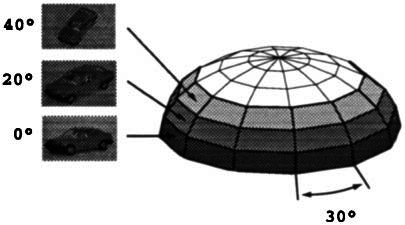
First consider the offline (training) steps. For a selected set of objects \(\{o_i\}\) to be recognized, and of viewpoints \(\{p_j\}\), we acquire images. Each of these images is then normalized to the same size and average brightness.
Now lets rewrite each image as a vector, say using raster ordering, to create image vectors \(x_{ij}\) of dim(N). So for instance, for a 512x512 image, N=512*512=262144. There will be \(N_x\) = (number of objects)x(number of viewpoints) such image vectors \(x_{ij}\).
Let \(\bar{x}\) be the average image vector
\(\bar{x}=(1/N_x)(\sum_{ij} x_{ij})\)
Define the vector X by concatenating the vectors \((x_{ij}-\bar{x})\) as column vectors. Then the covariance matrix of the image set \(\{x_{ij}\}\) is defined as
\(Q = XX^T\)
Note that dim(Q)=NxN, so for instance in a 512x512 image case with N=262144, Q is a 262144x262144 matrix with \(2^{18} \times 2^{18}=2^{36}\) or about 68 giga-elements.
The principal components of the image set \(\{x_{ij}\}\) are then the eigenvectors of Q, ordered in descending order of the magnitudes of their eigenvalues.
Since Q is symmetric and positive semi-definite (\(x^*Mx \ge 0\)), its eigenvectors will be orthogonal and can be considered normalized. Also, its eigenvalues will be non-negative.
The fractional mean square error in projecting \(\{x_{ij}\}\) into the subspace spanned by the first m principal components is
\(\text{FMSE} = \sum_{i>m} λ_i^2 / \sum_{j<=N} λ_j^2\)
where \(λ_1, λ_2 ,..., λ_N\) are the eigenvalues in descending order (largest first).
Eg: Consider an N=4 pixel image set with eigenvalues
\(λ_1=7, λ_2=3, λ_3=2, λ_4 =1\).
Then if we project the images into the 1-D subspace spanned by just its first principal component (first eigenvector), the fractional square error will be
\(\text{FMSE} = (3^2+2^2+1^2)/(7^2+3^2+2^2+1^2) =\)
\(= 14/63 = 0.222\)
So the fractional average error will be \(\sqrt{\text{FMSE}}\) or .471. Thus projecting from 4-D to 1-D we will lose about half the original image information.
Note: the projection of a vector x into the 1-D subspace spanned by the eigenvector \(e_1\) is the best approximation of x as \(a e_1\), where the coefficient vector a minimizes the error \(||x - a e_1||\).
If we project into a 2-D subspace of the first two eigenvectors,
\(\text{FMSE} = (2^2+1^2)/(7^2+3^2+2^2+1^2) = 0.0794\)
and the fractional average error will be \(\sqrt{.0794}\) or .28. So we will have lost about a quarter of the image information in projecting into 2-D.
The projection of a vector x into the 2-D subspace spanned by the eigenvectors \(e_1\) and \(e_2\) is the best approximation of x as \(a_1 e_1 + a_2 e_2\), where the coefficients \(a_1\) and \(a_2\) minimize the error \(||x- (a_1 e_1+a_2 e_2)||\).
Based on the eigenvalues (λ's) we compute offline, we can determine the FMSE using only the first k principal components, for k=1,2,.. until the FMSE is sufficiently low for our error tolerance.
We select this k and this becomes the dimension of the principal component subspace we will use for approximating image vectors, the subspace spanned by the first k eigenvectors \(\{e_1,...,e_k\}\), also called the principal components of the training data set.
So given any image vector x, dim(x)=N, we approximate x by g, dim(g)=k, where
\(g = \sum_i g_i e_i\)
where the \(g_i\) are the scalar weights of the various eigenvectors in approximating x in the reduced space of dimension k<<N, which are given by the inner products of the pattern x with the eigenvectors:
\(g_i = x^Te_i\)
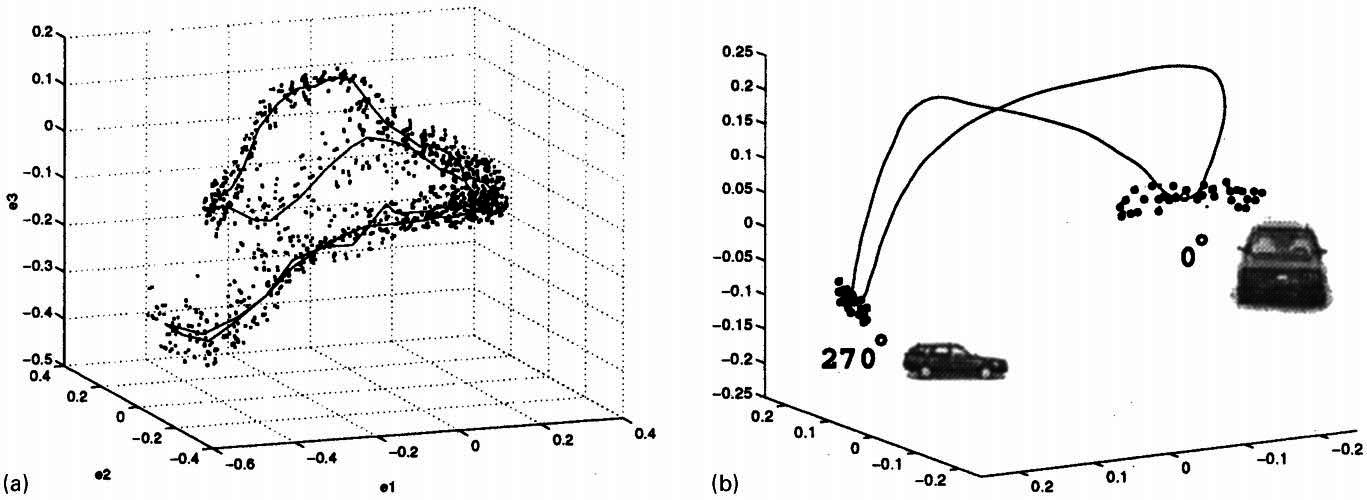
Now back to Borotshnig's active object recognition scheme. Besides the projection of a given vector into a selected k-dimensional principal component subspace, the other thing we must approximate offline is the probability density function of g, for each object \(o_i\) and pose \(p_j\), \(P(g|o_i,p_j)\).
This is done by taking a set of sample images with fixed \((o_i,p_j)\) but varying the lighting conditions, and fitting the resulting set of g-values by a Gaussian distribution.
\(P(g|o_i,p_j)\) can be used through Bayes' Law to determine posterior probabilities of object-pose hypotheses
\(P(o_i,p_j|g) = P(g|o_i,p_j)P(o_i,p_j)/P(g)\)
and the posterior object probabilities
\(P(o_i|g) = \sum_j P(o_i,p_j|g)\)
Thus, the most likely hypotheses \((o_i,p_j)\) and their scores \(P(o_i,p_j|g)\) can be determined by the recognition module online by projecting x down to g and using the offline probability database to get the hypothesis probabilities.
Marginalizing (summing the joint probabilities) over the poses yields the posterior probabilities of each object class given the image data g.
2. Data Fusion Module:
Using this Bayesian approach, data fusion becomes straightforward. Given a set of n image vectors \(\{x_1..x_n\}\) which project to their PCs \(\{g_1...g_n\}\),
\(P(o_i|g_1..g_n)=P(g_1..g_n|o_i)P(o_i)/P(g_1..g_n)\)
Lets determine this overall probability recursively assuming class-conditional independence
\(= P(g_1..g_{n-1}|o_i)P(g_n|o_i)P(o_i)/P(g_1..g_n)\)
\(= P(o_i|g_1..g_{n-1})P(o_i|g_n)P(o_i)/D\)
where
\(D = P(g_1..g_n)/(P(g_1..g_{n-1})P(g_n))\)
3. Decision module:
Decide \(o_i\) at time n if
\(i=\text{arg max} P(o_i|g_1..g_n)\)
and
\(P(o_i|g_1..g_n) > T\)
where T is a preselected threshold. So for instance if you require P(error)<5% you would set T=0.95+V, where V>0 is chosen to correct for sampling error in estimating the various probabilities.
4. Where do we look next?
Define the uncertainty in the object recognition task at time n as the entropy
\(H(O|g_1..g_n) = - \sum_i P(o_i|g_1..g_n) \log P(o_i|g_1..g_n)\)
of the prob density function of the random variable O where \(O=o_i\) if and only if the object class is i.
Now for each candidate change in the camera parameters we can determine the expected reduction in the entropy. This expected reduction depends on the \(\{P(o_i,p_j|g_1..g_n)\}\), the current hypothesis probabilities. For instance, if there are two very probable hypotheses and there is a way to change camera parameters to eliminate one or the other, that next-look with have a low expected entropy.
Their approach to view planning is to select the next view (camera parameters) which minimizes the expected entropy. See (9)-(11) in the paper for details.
5. Gaze control module
A control strategy to implement the physical motion, i.e. the view planning outcome. Not of interest here.
Strengths and Limitations of the Borotschnig approach
Strengths
A major strength is that it is a complete end-to-end active vision OR system based on well understood mathematical tools (PCA, Bayesian scoring, entropy).
Another strength is that it is domain-independent, and the database can be incrementally updated. In addition, Borotshnig's procedure does not require segmentation preprocessing, so the matching of test data is fast.
Limitations
A major problem with applying PCA to OR is that it is highly sensitive to object location in the object plane. Shifting the image radically changes the PCs.
Principal component analysis guarantees that the images in the training set, and images very similar to them, can be recognized using just a few principal components. But if an object is shifted in an image, like the test image above, its MS error compared to the corresponding image in the training set will be large, and the principal components will not be effective at capturing the test image, thus OR based on them will likely fail. Position counts!
In general, PCA is not invariant under affine transformations, of which pure translation is the most difficult to avoid. But rotation and scaling also must either be forbidden by tightly controlling the imaging environment, or otherwise be somehow compensated.
PCA is not invariant under lighting changes either. So large scale lighting changes will confound a PCA OR scheme.
Finally, it should be noted that PCA is a global rather than local matching procedure. This leads to problems with occlusion and clutter as Nelson discusses in the context of local vs. global keys.
These difficulties can each be addressed, but together probably limit the application of the method to highly constrained domains, like automated part inspection or "toy" problem domains.
A good approach to (relatively) unconstrained, natural-vision active OR has yet to be discovered. This is a great challenge for the next generation of researchers in the computer vision field!